When we make a decision every day, we often consult several people and comprehensively adopt their opinions. So is it possible to copy this idea into the field of machine learning and create multiple models to synthesize the results? Synthesizing is, of course, viable, and this idea is called the ensemble method.
Ensemble method
The ensemble method itself is not a specific method or algorithm, but an idea for training machine learning models. It has only one meaning, which is to train multiple models and then aggregate their results.
According to this idea, the industry has derived three specific methods, namely Bagging, Boosting, and Stacking.
Bagging Bagging is the abbreviation of bootstrap aggregating. We literally have a hard time understanding its meaning. We only need to remember this name. In the Bagging method, we will create K data sets by putting back random sampling. For each data set, there may be some single samples repeated, or some samples have never appeared, but overall, the probability of each sample is the same.
After that, we use the sampled K data sets to train K models. The model here is not limited. We can use any machine learning square model. K models will naturally get K results. Then we adopt the method of democratic voting to aggregate these K models.
For example, suppose K=25, in a binary classification problem. Ten model predictions are 0, and 15 model predictions that are 1. Then the final prediction result of the entire model is 1, which is equivalent to the democratic voting of K models. The famous random forest is this way.
Boosting The idea of Boosting is very similar to Bagging. They are consistent with the sampling logic of the sample. The difference is that in Boosting, the K models are not trained simultaneously, but serially. Each model will be based on the results of the previous model when training, and pay more attention to the samples that are judged wrong by the previous model. Similarly, the sample will also have a weight, and the sample with the larger error judgment rate will have a larger weight.
And each model will be given different weights according to their different capabilities, and finally, all models will be weighted and summed instead of fair voting. Due to this mechanism, the efficiency of the model during training is also different. Because all models of Bagging are entirely independent, we can take distributed training. Each model in Boosting depends on the previous model’s effect, so it can only be trained in series.
Stacking Stacking is a method often used in Kaggle competitions, and its idea is straightforward. We choose K different models and then use cross-validation to train and predict on the training set. Ensure that each model produces a prediction result for all training samples. Then for each training sample, we can get K results.
After that, we create a second layer model, and its training features are these K results. In other words, the structure of the multi-layer model will be used in the Stacking method. The last layer of the model’s training features is the results of the upper layer model’s prediction. It is up to the model to train which model’s results are more worthy of adoption, and how to combine the strengths between the models.
The AdaBoost we introduced today, as the name suggests, is a classic Boosting algorithm.
Modeling Ideas
The core idea of AdaBoost is to build a robust classifier through some weak classifiers by using the Boosting method.
We all understand the robust classifier: the model with reliable performance, so how should the weak classifier be recognized? The strength of the model is defined relative to the random result. The better the model than the random outcome, the more reliable it is its performance. From this point of view, a weak classifier is a classifier that is only slightly stronger than a random result. Our goal is to design the weights of samples and models so that the best decisions can be made, and these weak classifiers can be synthesized into the effects of robust classifiers.
First, we will assign a weight to the training samples. In the beginning, the weights of each sample are equal. A weak classifier is trained based on the training samples, and the error rate of this classifier is calculated. Then train the weak classifier again on the same data set. In the second training, we will adjust the weight of each sample. The correct sample weight will be reduced, and the wrong sample weight will be increased.
Similarly, each classifier will also be assigned a weight value, the higher the weight, the greater its speech power. These are calculated based on the error rate of the model. The error rate is defined as D over D’.
D here means that the data set represents the set of classification errors, which is equal to the number of samples in the error classification divided by the total number of samples.
With the error rate, we can get it according to the following formula.
After we got it, we used it to update the weight of the sample, and the weight of the correct classification was changed to epsilon.
The weight of the misclassified sample is changed to the delta.
In this way, all our weights have been updated, which completes a round of iterations. AdaBoost will repeatedly iterate and adjust the weights until the training error rate is 0, or the number of weak classifiers reaches the threshold.
Source Code
First, let’s get the data. Here we choose the breast cancer prediction data in the sklearn dataset. Like the previous example, we can directly import it and use it, which is very convenient:
import numpy as np
import pandas as pd
from sklearn.datasets import load_breast_cancer

breast = load_breast_cancer()
X, y = breast.data, breast.target
# reshape
y = y.reshape((-1, 1))
Next, we split the data into training data and test data, this is also a common practice without any difficulty:
from sklearn.model_selection import train_test_split

X_train, X_test, y_train, y_test = train_test_split(X, y, test_size=0.2, random_state=23)
In the AdaBoost model, the weak classifier we choose is the stump of the decision tree. The so-called tree stump is a decision tree with a tree depth of 1. The tree depth of 1, no matter how we choose the threshold, we will not get particularly good results, but because we still select the threshold and features, the result will not be too bad, at least better than random selection. So this guarantees that we can get a weak classifier that is slightly better than random selection, and its implementation is straightforward. Before we implement the model, let’s implement several auxiliary functions.
These three functions should not be difficult to understand. In the first function, we calculated the error of the model. Since each of our samples has its weight, we weight and sum the errors. The second function is the prediction function of the stump classifier, the logic is straightforward, and the size is compared according to the threshold. There are two cases here. It is possible that the sample smaller than the threshold is a positive example, or that the sample larger than the threshold is a positive example, so we need a third parameter to record this information. The third function is a function that generates a threshold. Since we don’t need the stump performance to be particularly useful, we don’t need to traverse all the threshold values and divide the range of features into ten segments.
Next is the generation function of a single stump, which is equivalent to selecting features in the decision tree to split the data. The logic is similar, and only a slight modification is required.
def build_stump(X, y, weight):
    m, n = X.shape
    ret_stump, ret_pred = None, []
    best_error = float('inf')

    for i in range(n):
        for j in get_thresholds(X, i):
            for c in ['lt', 'gt']:
                pred = stump_classify(X, i, j, c).reshape((-1, 1))
                err = loss_error(pred, y, weight)
                if err < best_error:
                    best_error, ret_pred = err, pred.copy()
                    ret_stump = {'idx': i, 'threshold': j, 'comparator': c}
    return ret_stump, best_error, ret_pred

def adaboost_train(X, y, num_stump):
    stumps = []
    m = X.shape[0]
    weight = np.ones((y_train.shape[0], 1)) / y_train.shape[0]
    for i in range(num_stump):
        best_stump, err, pred = build_stump(X, y, weight)
        alpha = 0.5 * np.log((1.0 - err) / max(err, 1e-10))
        best_stump['alpha'] = alpha
        stumps.append(best_stump)

        for j in range(m):
            weight[j] = weight[j] * (np.exp(-alpha) if pred[j] == y[j] else np.exp(alpha))
        weight = weight / weight.sum()
        if err < 1e-8:
            break
    return stumps
After the stump generation is completed, the final part is the prediction. The whole forecasting process is still straightforward, it is a weighted sum process. It should be noted here that to highlight the wrongly predicted samples during training, the model has better capabilities and maintains the weight of the samples. However, during prediction, we do not know the weight of the prediction sample, so we only need to weigh the model’s results.
def adaboost_classify(X, stumps):
    m = X.shape[0]
    pred = np.ones((m, 1))
    alphs = 0.0
    for i, stump in enumerate(stumps):
        y_pred = stump_classify(X, stump['idx'], stump['threshold'], stump['comparator'])
        pred = y_pred * stump['alpha']
        alphs += stump['alpha']
    pred /= alphs
    return np.sign(pred).reshape((-1, 1))
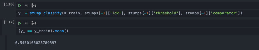
Our entire model is completed, let us first examine the performance of a single stump on the training set:
It can be seen that the accuracy rate is only 0.54, which is only slightly better than random prediction.
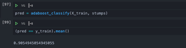
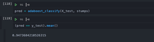
However, after synthesizing the results of 20 stumps, we can get an accuracy of 0.9 on the training set. In the prediction set, it performs better, and the accuracy rate is close to 0.95! The measurement is slightly better.
This is because in AdaBoost, each classifier is a weak classifier, and it cannot overfit at all. After all, the performance in the training set is inferior, which ensures that the classifier learns all the generalizations. The ability applies to the training set and a significant probability of the test set. This is also one of the most significant advantages of the integration method.